实战环节 上一期对所拥有的数据做了个表达定量并生成了表达矩阵,现在进入差异分析的环节
差异分析 本次做差异分析所使用的工具是基于python的omicverse库
该模块的其安装方法也很简单,但需注意的是omicverse库必须在linux环境或windows系统的WSL环境下使用。
1 2 3 4 5 6 7 8 9 10 11 12 13 14 15 16 conda create -n omicverse python=3.10 conda activate omicverse conda install pytorch torchvision torchaudio pytorch-cuda=11.8 -c pytorch -c nvidia conda install pytorch torchvision torchaudio cpuonly -c pytorch conda install pyg -c pyg conda install omicverse -c conda-forge
本次分析选用的数据集是GSE118916。从GEO数据库中进行下载:
使用omicverse进行常规的差异基因表达分析 1 2 import pandas as pdimport os
1 2 3 4 5 6 7 8 9 10 11 12 13 14 expressionData = pd.read_csv("expression_data.csv" , encoding='UTF-8' ) indexNum = 0 indexList = [] for i in list (expressionData.iloc[:,0 ]): if '---' == i: indexList.append(indexNum) indexNum += 1 expressionData_Drop = expressionData.drop(indexList) expressionData_Drop
输出:
Gene Symbol GSM3351221 GSM3351222 GSM3351223 GSM3351224 GSM3351225 GSM3351226 GSM3351227 GSM3351228 … GSM3351240 GSM3351241 GSM3351242 GSM3351243 GSM3351244 GSM3351245 GSM3351246 GSM3351247 GSM3351248 GSM3351249 0 HIST1H3G 4.333162 3.393413 3.202298 3.273934 3.149646 3.371994 3.627498 3.046871 3.969594 … 3.623850 3.664705 3.340904 3.602020 3.331657 3.392765 3.493841 3.487211 3.391482 1 HIST1H3G 5.509134 5.405715 5.184302 4.883117 4.896176 5.113827 5.167449 5.110204 5.556905 … 4.851287 5.397218 5.153698 5.201280 4.851287 5.374734 5.276653 5.188680 5.140900 2 HIST1H3G 4.686904 3.871414 3.724224 3.397720 3.615277 3.841320 4.325271 3.560210 4.341479 … 3.992363 3.987619 3.687451 3.855043 3.694976 3.766741 3.963058 4.101157 3.854747 3 TNFAIP8L1 4.361757 4.285916 4.377757 5.367287 6.018805 4.888754 4.743503 4.430155 4.498028 … 3.740284 3.791165 4.206512 3.795124 3.853014 3.782595 3.757001 3.663455 3.869301 4 OTOP2 4.692442 4.467624 4.430727 4.132381 4.265175 4.237638 4.287581 4.428147 4.352447 … 4.834237 4.873393 4.521720 4.899339 5.179813 4.866155 5.235878 4.829041 4.766776 … … … … … … … … … … … … … … … … … … … … … 49297 GAPDH 2.250415 2.196336 2.188453 2.140965 2.205614 2.172010 2.216602 2.180626 2.197528 … 2.311198 2.319124 2.243291 2.354154 2.397206 2.348041 2.317698 2.321311 2.272872 49298 STAT1 2.349588 2.322962 2.277523 2.217424 2.293500 2.242945 2.283375 2.278833 2.299161 … 2.439090 2.465033 2.348560 2.472626 2.507350 2.452186 2.461888 2.474203 2.423064 49299 STAT1 2.671896 2.611722 2.612591 2.468304 2.585089 2.535129 2.606042 2.542626 2.584898 … 2.811227 2.805426 2.675989 2.881790 2.842771 2.828554 2.840772 2.815630 2.776199 49300 STAT1 3.041021 3.000218 2.956512 2.836378 2.925315 2.865108 2.960598 2.930377 2.947940 … 3.221686 3.264126 3.072335 3.282286 3.309083 3.238734 3.269109 3.202032 3.186877 49301 STAT1 3.521169 3.519029 3.485920 3.299582 3.402691 3.347042 3.427732 3.405621 3.408984 … 3.757983 3.837290 3.611317 3.841599 3.827958 3.830761 3.752328 3.749842 3.681698
1 2 3 4 5 6 7 8 expressionData_Drop.set_index(["Gene Symbol" ], inplace=True ) import omicverse as ovimport scanpy as scimport matplotlib.pyplot as pltov.ov_plot_set()
输出:
1 2 3 4 🔬 Starting plot initialization... 🧬 Detecting CUDA devices… 🚫 No CUDA devices found ✅ plot_set complete.
1 2 3 4 5 6 7 8 9 10 dds = ov.bulk.pyDEG(expressionData_Drop) dds.drop_duplicates_index() print ('... drop_duplicates_index success' )dds.normalize() print ('... estimateSizeFactors and normalize success' )
输出:
1 2 ... drop_duplicates_index success... estimateSizeFactors and normalize success
1 2 3 4 5 6 7 treatment_groups=['GSM3351220' ,'GSM3351221' ,'GSM3351222' ,'GSM3351223' ,'GSM3351224' ,'GSM3351225' ,'GSM3351226' ,'GSM3351227' ,'GSM3351228' ,'GSM3351229' ,'GSM3351230' ,'GSM3351231' ,'GSM3351232' ,'GSM3351233' ,'GSM3351234' ] control_groups=['GSM3351235' ,'GSM3351236' ,'GSM3351237' ,'GSM3351238' ,'GSM3351239' ,'GSM3351240' ,'GSM3351241' ,'GSM3351242' ,'GSM3351243' ,'GSM3351244' ,'GSM3351245' ,'GSM3351246' ,'GSM3351247' ,'GSM3351248' ,'GSM3351249' ] result_ttest=dds.deg_analysis(treatment_groups,control_groups,method='ttest' ) result_ttest.sort_values('qvalue' ).head()
输出:
1 2 3 ⚙️ You are using ttest method for differential expression analysis. ⏰ Start to calculate qvalue... ✅ Differential expression analysis completed.
Gene Symbol pvalue qvalue FoldChange MaxBaseMean BaseMean log2(BaseMean) log2FC abs(log2FC) size -log(pvalue) -log(qvalue) sig DMRTA1 3.372637e-17 6.773267e-13 0.715917 5.498099 4.453653 2.154989 -0.482136 0.482136 0.071592 16.472030 12.169202 sig CAPN13 1.526491e-15 1.532826e-11 0.849719 6.694391 6.051985 2.597408 -0.234943 0.234943 0.084972 14.816306 10.814507 sig LNX1 3.725194e-15 2.493769e-11 0.763073 6.469154 5.483045 2.454977 -0.390108 0.390108 0.076307 14.428851 10.603144 sig CAPN9 5.643624e-15 2.833522e-11 0.667939 7.792100 6.190386 2.630029 -0.582212 0.582212 0.066794 14.248442 10.547673 sig CLDN12 7.299049e-15 2.931736e-11 0.903028 6.111705 5.725430 2.517384 -0.147158 0.147158 0.090303 14.136734 10.532875 sig
1 2 3 4 5 6 7 8 print (dds.result.shape)dds.result=dds.result.loc[dds.result['log2(BaseMean)' ]>1 ] print (dds.result.shape)输出: (14028 , 12 ) (14028 , 12 )
1 2 3 4 5 6 dds.foldchange_set(fc_threshold=-1 , pval_threshold=0.05 , logp_max=10 )
输出:
1 ... Fold change threshold: 0.16936119706053465
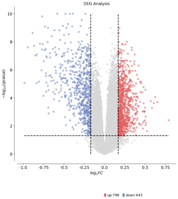
1 2 3 4 5 6 7 8 dds.plot_volcano(title='DEG Analysis' ,figsize=(10 ,10 ), plot_genes_num=0 ,plot_genes_fontsize=0 ,)
输出:
1 2 3 4 5 6 7 8 9 10 11 12 13 14 15 16 17 18 19 🌋 Volcano Plot Analysis: Total genes: 14028 ↗️ Upregulated genes: 798 ↘️ Downregulated genes: 643 ➡️ Non-significant genes: 12587 🎯 Total significant genes: 1441 log2FC range: -0.99 to 0.79 qvalue range: 6.77e-13 to 1.00e+00 ⚙️ Current Function Parameters: Data columns: pval_name='qvalue', fc_name='log2FC' Thresholds: pval_threshold=0.05, fc_max=0.16936119706053465, fc_min=-0.16936119706053465 Plot size: figsize=(10, 10) Gene labels: plot_genes_num=0, plot_genes_fontsize=0 Custom genes: None (auto-select top genes) 💡 Parameter Optimization Suggestions: ✅ Current parameters are optimal for your data! ────────────────────────────────────────────────────────────
1 <AxesSubplot: title={'center': 'DEG Analysis'}, xlabel='$log_{2}FC$', ylabel='$-log_{10}(qvalue)$'>
使用 DEseq2 进行差异表达分析 借助 pyDEseq2,可以像 R 语言那样分析差异表达基因
1 2 3 4 5 6 7 8 expressionData_int = expressionData_Drop.astype(int ) dds_int = ov.bulk.pyDEG(expressionData_int) dds_int.drop_duplicates_index() print ('... drop_duplicates_index success' )
输出:
1 ... drop_duplicates_index success
1 2 3 4 5 6 7 treatment_groups=['GSM3351220' ,'GSM3351221' ,'GSM3351222' ,'GSM3351223' ,'GSM3351224' ,'GSM3351225' ,'GSM3351226' ,'GSM3351227' ,'GSM3351228' ,'GSM3351229' ,'GSM3351230' ,'GSM3351231' ,'GSM3351232' ,'GSM3351233' ,'GSM3351234' ] control_groups=['GSM3351235' ,'GSM3351236' ,'GSM3351237' ,'GSM3351238' ,'GSM3351239' ,'GSM3351240' ,'GSM3351241' ,'GSM3351242' ,'GSM3351243' ,'GSM3351244' ,'GSM3351245' ,'GSM3351246' ,'GSM3351247' ,'GSM3351248' ,'GSM3351249' ] result = dds_int.deg_analysis(treatment_groups,control_groups,method='DEseq2' )
输出:
1 2 3 ⚙️ You are using DEseq2 method for differential expression analysis. ⏰ Start to create DeseqDataSet... Using None as control genes, passed at DeseqDataSet initialization
1 2 3 4 5 6 7 8 9 10 Fitting size factors... ... done in 0.05 seconds. Fitting dispersions... ... done in 0.65 seconds. Fitting dispersion trend curve... ... done in 0.22 seconds. Fitting MAP dispersions...
1 logres_prior=1.5254760032591015, sigma_prior=1.4514357345950912
1 2 3 4 5 6 7 8 9 10 11 ... done in 1.82 seconds. Fitting LFCs... ... done in 0.77 seconds. Calculating cook's distance... ... done in 0.02 seconds. Replacing 0 outlier genes. Running Wald tests...
1 2 3 4 5 6 7 8 9 10 11 12 13 14 15 16 17 18 19 20 21 22 23 24 25 26 27 28 29 30 31 Log2 fold change & Wald test p-value: condition Treatment vs Control baseMean log2FoldChange lfcSE stat \ Gene Symbol COX3 /// MYBPC3 /// SLC12A1 13.074116 0.001168 0.154571 0.007559 TPT1 13.007369 0.001171 0.154922 0.007558 ND4 13.007369 0.001171 0.154922 0.007558 ATP13A5 /// HARS 12.974036 -0.006246 0.155129 -0.040261 B2M 12.840421 -0.021317 0.155953 -0.136689 ... ... ... ... ... SSX1 1.300795 -0.072834 0.473870 -0.153699 C2orf83 1.300624 -0.221223 0.475017 -0.465715 CLCA3P 1.233980 -0.551375 0.494168 -1.115764 UGT2B11 1.200886 -0.484293 0.501002 -0.966649 RAD21L1 1.233900 -0.076840 0.486072 -0.158084 pvalue padj Gene Symbol COX3 /// MYBPC3 /// SLC12A1 0.993969 0.997498 TPT1 0.993969 0.997498 ND4 0.993969 0.997498 ATP13A5 /// HARS 0.967885 0.997498 B2M 0.891277 0.997498 ... ... ... SSX1 0.877847 NaN C2orf83 0.641419 NaN CLCA3P 0.264523 NaN UGT2B11 0.333719 NaN RAD21L1 0.874391 NaN [20083 rows x 6 columns] ✅ Differential expression analysis completed.
1 ... done in 1.17 seconds.
1 2 3 print (result.shape)result=result.loc[result['log2(BaseMean)' ]>1 ] print (result.shape)
输出:
1 2 3 4 dds_int.foldchange_set(fc_threshold=-1 , pval_threshold=0.05 , logp_max=10 )
输出:
1 ... Fold change threshold: 0.2874723264386634
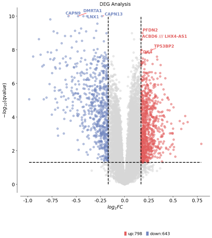
1 2 3 dds.plot_volcano(title='DEG Analysis' ,figsize=(10 ,10 ), plot_genes_num=8 ,plot_genes_fontsize=12 ,)
输出:
1 2 3 4 5 6 7 8 9 10 11 12 13 14 15 16 17 18 19 🌋 Volcano Plot Analysis: Total genes: 14028 ↗️ Upregulated genes: 798 ↘️ Downregulated genes: 643 ➡️ Non-significant genes: 12587 🎯 Total significant genes: 1441 log2FC range: -0.99 to 0.79 qvalue range: 6.77e-13 to 1.00e+00 ⚙️ Current Function Parameters: Data columns: pval_name='qvalue', fc_name='log2FC' Thresholds: pval_threshold=0.05, fc_max=0.16936119706053465, fc_min=-0.16936119706053465 Plot size: figsize=(10, 10) Gene labels: plot_genes_num=8, plot_genes_fontsize=12 Custom genes: None (auto-select top genes) 💡 Parameter Optimization Suggestions: ✅ Current parameters are optimal for your data! ────────────────────────────────────────────────────────────
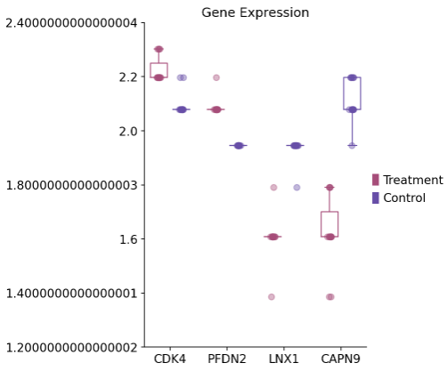
1 2 3 4 dds_int.plot_boxplot(genes=['CAPN9' ,'LNX1' ,'PFDN2' ,'CDK4' ],treatment_groups=treatment_groups, control_groups=control_groups,figsize=(4 ,6 ),fontsize=12 , legend_bbox=(1 ,0.55 ))
输出:
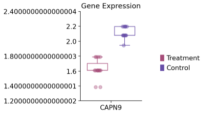
1 2 3 4 dds_int.plot_boxplot(genes=['CAPN9' ],treatment_groups=treatment_groups, control_groups=control_groups,figsize=(2 ,3 ),fontsize=12 , legend_bbox=(2 ,0.55 ))
输出: